Home About us Contact us Protuner Loop Analyser & Tuner Educational PDFs Loop Signatures Case Histories
Michael Brown Control Engineering CC
Practical Process Control Training & Loop Optimisation
LOOP SIGNATURE 27
TUNING - PART 5
SWAG TUNING OF SIMPLE INTEGRATING PROCESSES
The chief control engineer of one of the largest petro-chemical refineries in South Africa sent me an email after a course in his plant. He wrote that he had found the section on swag tuning of simple integrating processes one of the most informative of the whole course. After the course he went out into his plant for a couple of days and personally optimised 16 level controls. He found that that the originally tuning in all of them was appalling. He decided to try tuning them using the methods covered in this section, even though he had a Protuner, and he found to his delight that he obtained excellent results.
As a matter of interest this section arose from a course I was giving at a remote diamond mine in Namibia, quite a few years ago. Their processing plant was then quite primitive as compared to the modern one they now have, and there was only one self-regulating loop that was a density control. All the rest of the loops were tank levels. The delegates on the course appealed to me to offer them a simple method of tuning level loops, as they would never have been able to justify expenditure for a loop analysis and tuning package. The following is what we developed in that session.
In the previous three articles in this Loop Signature series, we were looking at SWAG tuning of simple self-regulating processes. Now we go on to deal with simple integrating processes like level. Once again I must stress that this is for simple integrating processes. When it comes to tuning integrators with complex dynamics, such as very long dead-times, or with leads, or large lags, you really do need to use a good tuning package like the Protuner.
Very few people have any real understanding of the characteristics of integrating processes, and how to go about tuning them. This is because the majority of control practitioners have not been taught about the differences between self-regulating and integrating processes. In most plants the majority of loops are self-regulating processes, which most people find easier to tune by trial and error, and they develop a feel for them. They then try and use that knowledge to tune integrating processes. This is where the main problem comes in, because integrating processes work very differently to self-regulating processes, and are tuned completely differently.
As a result we find that the vast majority of integrating processes in plants are tuned all wrong, and hence operate badly. Typically most are tuned extremely slowly, often with large over and undershoots on setpoint step changes, followed by a very slow damped cycle that sometimes takes hours to die out.
In my courses I always refer to the section on tuning simple integrating processes by a SWAG method as a “brain washing” exercise, as we need to change the mind-set that most people have of tuning. This will be illustrated as the article progresses.
Let us imagine we have been asked to tune the level control on a particular tank in your plant. The control requirements are:
1. No cycling is permissible. This is the most important requirement.
2. The response must be as fast as possible. Only one overshoot is permissible on a step change in setpoint.
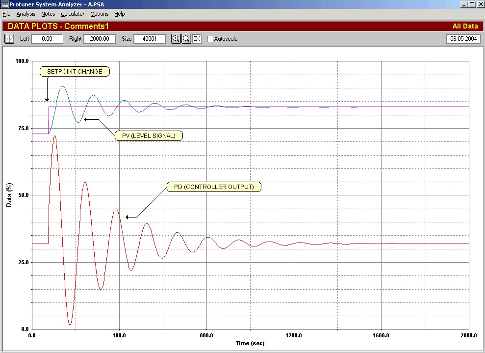
We go out to the loop, and perform a closed loop test as found. (Set point step change test using the existing tuning settings). The result is shown in Figure 1. It is pretty bad with huge overshoots and undershoots with a damped cycle that takes nearly half an hour to die out. We can see why the process people want something done about it if they don’t want cycling. Incidentally I encounter responses like this on many level controls in the majority of plants I work in.
Figure 1
Now assuming we have not been taught much about integrating processes, we will try and tune the loop the way we would a self-regulating process. As the most important requirement is no cycling allowed, we will first try and stop the existing cycle.
How do we do this? Well all our experience on self-regulating processes has taught us that if the response is too fast then we must reduce the controller gain (KP), i.e. increase the proportional band.
Going into the controller parameter settings we find that the person who had previously tuned the controller had set in a KP of 1 and an integral of 5 seconds/repeat. The controller has a series algorithm.
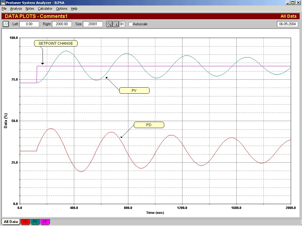
Being determined to really get rid of the cycling we reduce the gain by a factor of 10, and set the KP equal to 0,1. Another test is then done with a step change of setpoint. This is shown in Figure 2.
Figure 2
To our horror the cycling has actually got much worse. After nearly 40 minutes it is still cycling away, and this will obviously go on for a long while! This is the exact opposite of what we expected to happen, and our self –confidence is suddenly badly shaken as we don’t understand why it has got worse. What can be done?
The answers lie in the following SWAG tuning rules for simple integrating processes:
SWAG Tuning Rule No 1 for Simple Integrating Processes: Switch off I and D (if it has been used), and use P only control.
SWAG Tuning Rule No 2 for Simple Integrating Processes: Make setpoint changes and establish the closed loop response to you want by trial and error by adjusting Kp (proportional gain).
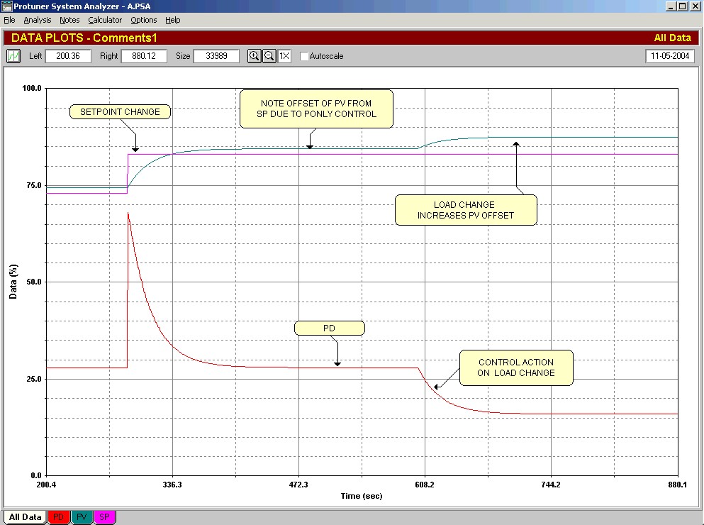
A test showing the response to a setpoint change with a Kp of 4 is shown in Figure 3. The control is typical of a P only control scheme.
Figure 3
The Loop Signature article entitled “Digital Controllers - Part 3 - the P Term” published in October 2001, showed how P only control generally results in the measurement being offset from setpoint. Adjusting the manual bias in the controller can reset the offset. However any load change will result in a fresh offset. As level controls usually have relatively high gains the offset may be relatively small and might not be a problem. (Offset cannot be larger than the proportional band).
Higher gain in the P only controller will give the advantages of smaller offset and also faster control response. However the higher the gain the more the output of the controller (PD) moves around, thus leading to a more valve wear and hence a shorter life. There is also very often a high noise amplitude in level measurements. This will be amplified through the P term of the controller; again increasing valve wear. Therefore when tuning integrating processes like levels, one has to carefully balance valve life against control performance.
In the example we are tuning here, as mentioned above, the control response shown in Figure 3 is with a Kp of 4. In actual fact much better control and less offset could be obtained with higher gains of typically 12 or 20, but in this case let us imagine we are happy with the control response and don’t wish to work the valve too hard, so we will stay with the gain of 4.
SWAG Tuning Rule No 3 for Simple Integrating Processes: Once you are happy with the response, and if the offset is not a problem, then the job is done. Leave the controller like that.
Note: Integrating loops are in actual fact better without an I term in the controller. There are two reasons for this. The first as mentioned in previous articles, is that any hysteresis on a valve on an integrating process that is controlled with P + I control will result in continuous cycling. The second reason is that the I term introduces a second integral term into the combined loop process transfer function, and prevents perfect pole cancellation tuning from being achieved.
If however the offset is unacceptable, which may be the case here, as with a P gain of 4 (i.e. a proportional band of 25%), relatively large offsets would result if big load changes occur, then one must use the I term.
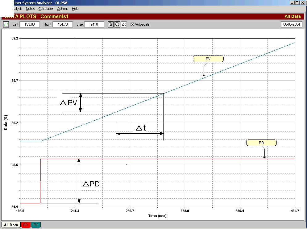
SWAG Tuning Rule No 4 for Simple Integrating Processes: If you need to use the I term because the offset is unacceptable, then the next step is to determine the Process Gain.
Figure 4
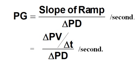
This was covered in a previous Loop Signature. To recap, and also referring to Figure 4, the process gain of an integrating process is given by:
On our loop the PG works out as 0.01/second.
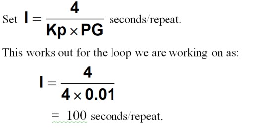
SWAG Tuning Rule No 5 for Simple Integrating Processes:
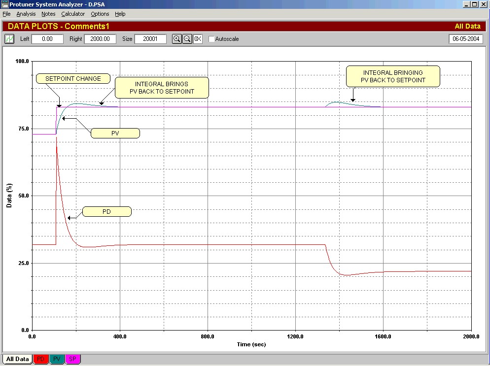
The recording of a closed loop step test with this tuning is shown in Figure 5. It can be seen that the control is working very well with good recovery from load changes.
Figure 5
SWAG Tuning Rule No 6 for Simple Integrating Processes: The SWAG formula for the I term given in Rule 5 above is very approximate and is relatively safe. In most cases if you feel the response is too slow, you can reduce the integral by trial and error. As you do so, you will find the overshoot will increase on setpoint changes, but the response to load changes will be faster. However do not let get the response get too cyclic.
I generally prefer to tune integrating processes so that the response to setpoint changes result in only one overshoot
To change your mind set when tuning integrating processes:
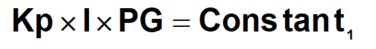
The little equation given in Rule 5 is really a SWAG type of formula, but it gives excellent results. Moving the denominator on the right side to the left hand side gives us:
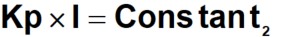
In most cases PG is also a constant. Moving it to the right hand side results in an equation:
This means that if you wish to change the response by altering Kp, then you need to change I proportionally. Thinking a bit further about this we see that the higher the gain we put in, the faster we can make the integral. This goes completely against all our “gut” feelings we have established by years of tuning mostly self-regulating processes. However its true, and it works well within reasonable boundaries. There are a lot of advantages for using higher gains on integrating processes, which generally need tuning with relatively slow integrals, so being able to speed up the integral is great.
Conversely if you really must have a slow response and need to reduce Kp, then you must increase the I term proportionally.
Be careful that the process gain is in fact constant. If it varies, which it will do for example on non-uniform tanks, or gravity feed tanks, then you must also take it into account. If the PG varies then at least one, or both of the other two terms must change to keep the constant the same.