Home About us Contact us Protuner Loop Analyser & Tuner Educational PDFs Loop Signatures Case Histories
Michael Brown Control Engineering CC
Practical Process Control Training & Loop Optimisation
CONTROL LOOP CASE HISTORY 139
IMPORTANCE OF MEASUREMENTS AND DYNAMICS
One of the first laws of process control states that you cannot control what you cannot measure. However although instrument practitioners all know this, they very often apparently forget it.
I think this is largely due to the fact that most modern measuring instrumentation falls into the “smart” category, which means they are computerized, and one of the most common fallacies I find in the world of instrumentation and control is the apparent belief that anything working with a computer inside it must be right.
An even bigger common fallacy is that if a control loop is not working properly then all you have to do is tune the controller. Many people booked on my courses tell me on arrival that they have come to attend the tuning course. I immediately tell them that they are on the wrong course. My courses deal with loop optimisation, and tuning is only a tiny part of them. In fact in about 50% cases of problem loops, tuning is a complete waste of time without first sorting out the loop problems which involves a thorough analysis of the components of the loop and gaining full understanding of all the control requirements. Furthermore it is essential that one uses proper analytical and tuning software if one is to perform optimisation properly and efficiently.
The measurement is one component in the loop, and it is the one that is most frequently ignored. I have come across cases like a person spending over 6 hours trying to tune a controller to get the control working, when in fact there was a blocked impulse line leading from the orifice plate to the transmitter. Another memorable case was a group of control engineers who spent several days installing feedforward on a boiler drum level control system to overcome particular problem, only to find out at a little later that the drum level measurement was completely wrong due to incorrect installation of the measuring instrument.
Another pet distrust of mine is the use of ultrasonic level transmitters in certain applications for which they are not suitable.
I also find that many users have very little idea of how their measuring instruments work, and invariably have received no training on them. I have lost count of the times I have asked plant personnel to show me the instruction manual on certain instruments, only to be told that they have lost or do not have a manual.
Another thing I find fairly often that people have forgotten really basic things about correct usage and installation of really basic measuring devices, and in particular orifice plate flow measurement. This is something that goes back literally for hundreds of years, and the theory was first published by Bernoulli in 1738. I am sure that this one of the first thing taught to budding instrumentation and control practitioners when they first start their studies. Orifice plate measurement is still regarded as one of the primary methods of flow measurement and is still used as a standard for metering in custody flow applications. The reason for this is that many countries and authorities have standard relating to this method of measurement based on many years of empirical research as well the basic theory.
It is however not very accurate and installation has to be performed according to very strict rules. For example British Standard 1042 states that a properly installed and calibrated orifice plate measuring system is accurate to ±2% of full scale over a 3:1 range. In practice over many decades, people in the control field use it with confidence up to a 4:1 range. However it is a well known fact that the readings can be completely unreliable below the lower limit of 25%, and should not be used or relied on.
Many plants particularly in the oil and chemical industries make extensive use of orifice plate measurement due to the fact they deal with non-conductive fluids and thus cannot use the more popular and far more accurate magnetic flowmeter type measurements. These plants usually use high end grade measuring transmitters and control equipment and do not skimp on cheaper alternatives such as often found in industries like mining. They also usually have relatively high grade technical staff.
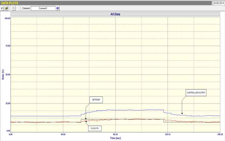
In spite of this I often find flow controls in these plants where they are working way below the 25% mark. Figure 1 shows a closed loop test performed recently on a flow loop in a refinery. This is one of the worst cases I have seen of incorrect use of the measuring system. The setpoint was usually at 8% of the measuring range. It is amazing that nobody in these plants seem to be aware that measurements like this are probably completely incorrect, and yet there is always consternation when plant balances don’t correlate.
Fig 1.
The second example in this article is to emphasis the importance of identifying the dynamics in a process when tuning a controller. This is one of the 6 most important points I always stress in my courses on loop optimization.
One of the most interesting types of dynamics that can occur on some integrating processes is a first order lead/lag. Full information on this can be found the articles LSp2-20, and LSp2-21 which was published in my collection of articles entitled “Dynamics of More Complex Processes”.
The main characteristic of these dynamics is that there is an initial fast response to a step change on the input of the process, before the process settles into the normal constant ramp typical of integrators. This type of response is most typically found on the pressure control of drier stages on paper machines. However it can also occur in places where you least expect it.
In general these processes are usually terribly badly tuned, as instability can easily arise with incorrect tuning. This is because of the lead, which tends to frighten people. I have often heard Operators express unease when we optimise loops with leads, whether positive or negative. They say: “Be careful. This loop can run away very quickly!” As a result the tuning is usually extremely slow with extremely long integrals which are typically needed for integrating processes.
In fact, these processes actually exhibit both self-regulating and integrating characteristics. On a change the response reacts initially as a relatively fast self-regulating process and it then changes into an integrating process. There are various reasons for this depending on the type of process, and this is discussed fully in the above referenced articles.
The trick with positive lead integrators is to tune them on the initial self-regulating response, and ignore the integrating part that follows after.
The particular process that will be discussed here is the pressure control at the top of a distillation column. It is an extremely important control as the performance of the column is influenced by the pressure. The process people were complaining that the pressure did not remain constant under load changes, and took an extremely long time responding to such changes.
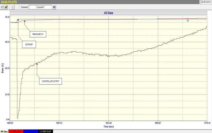
Figure 2 shows a closed loop test with the original tuning. Only very small set point changes were allowed so as not to disturb the column too much. The test confirms that the response of the control was extremely slow. Also of interest it can be seen that in the latter part of the test the pressure was slightly above setpoint and the controller was ramping up the output without being able to bring the pressure back down.
Fig 2.
The tuning in the controller was P = 22.5 and I = 10.1 minutes/repeat.
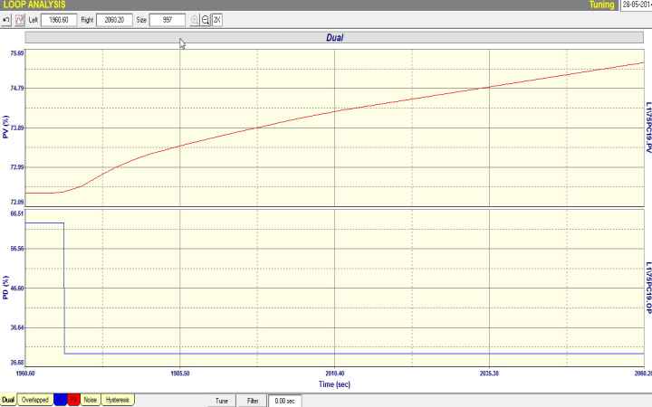
Figure 3 shows a portion of the the open loop step test. The first order positive lead, although not very large is seen by the initial relatively fast rise in pressure followed by the typical integrating ramp. (The lead is actually about 20 seconds.) What is not shown in the figure was that it was found that when the controller output moved up past about 75% the control had no further effect on the pressure. This is a serious problem as control of higher pressures is not possible.
Fig 3.
Tuning the controller over the first self-regulating portion of the test gave a tuning of P = 11 and I = 0.2 minutes/repeat. Note the integral has now been reduced by an amazing factor of 55 from the original tuning!
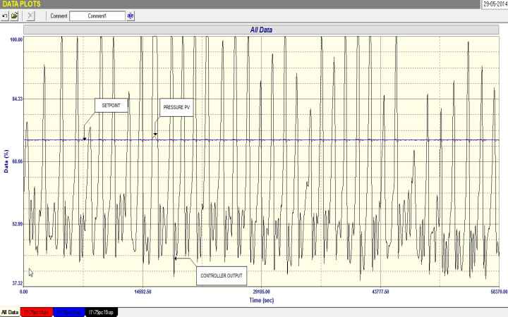
The new tuning worked amazingly well, being so much faster than the old. However in final closed loop testing over a period of some 16 hours it was observed that there was a load cycle with a period of approximately 28 minutes affecting the column, and causing an increase in pressure past the point where the valve could no longer control. Figure 4 shows the pressure control operating over this period. During “normal” periods it can be seen that the control was absolutely amazing, keeping the pressure at setpoint with almost zero variance. However when the load peaked the control could not hold the pressure.
Fig 4.
The main point I wish to stress in this example is how important it is to recognise dynamics present in a process so that the correct type of tuning can be applied for best control.