Home About us Contact us Protuner Loop Analyser & Tuner Educational PDFs Loop Signatures Case Histories
Michael Brown Control Engineering CC
Practical Process Control Training & Loop Optimisation
CONTROL LOOP CASE HISTORY 151
THE MYTHS SURROUNDING DEADTIME DOMINANT PROCESSES
The practice of industrial feedback control is one of the most misunderstood engineering disciplines in the world. The theory was developed by eminent mathematicians in the early 1900’s, and was based on highly mathematical principles which are extremely hard to apply practically in an industrial process plant without the right tools. Teaching is invariably almost entirely on the mathematics with no practical explanations. Most practitioners entering the field find they can’t use the theory, and develop their own “feelings’ on how to do things. Many of their beliefs are actually incorrect. As a result about 85% of all control loops worldwide are operating completely inefficiently in automatic. (This last statement is often hotly disputed by “experts” in the field, but after optimising many thousands of loops we stand fully behind it.)
Fallacies resound around the industry such as:
• Any control problem can be solved by tuning.
• Smart (computerised) measuring instruments and positioners must be right.
• You don’t need highly skilled people to make control systems work and particularly to tune controllers.
However the subject that seems to have the most misconceptions, and of which a lot of rubbish which is published on internet control discussion groups is how to control deadtime dominant processes.
A deadtime dominant process is defined as one where the deadtime is greater or equal to the dominant lag. One of the best examples of such a process is weigh feeder control on conveyor systems as typically used in mining applications. This is due to the fact that the measuring point is often very far away from the feeders.
Deadtime is the “bad guy” in feedback control as it introduces phase lag into the loop and can result in instability with bad tuning. (An interesting fact is that theoretically if a process has zero deadtime then you cannot make a loop unstable, irrespective of the tuning. Why I say “theoretically” is because in the real world there will always be some deadtime somewhere in the components of the control loop.)
Tuning of deadtime processes has always been a bit of a puzzle. In the original Ziegler-Nichols paper on tuning published in the early 1940’s they actually specifically mentioned that they couldn’t give tuning formulae for deadtime dominant processes.
In real life most of these processes are incredibly badly tuned.
However in actual fact if you think of it, we all know what to do when controlling long deadtime processes. I am sure that we have all experienced taking a shower and have had then experience where it takes a long time for the temperature to change after you have adjusted one of the taps. If you turn the tap too much then a deadtime later you suddenly freeze or else scald yourself. You then quickly learn to turn the taps a little at a time and then wait until the resultant change is felt. So what you have learnt is to slow the control down! So the secret of controlling these processes is to slow the control down.
The Golden Rule is: “The longer the deadtime, the slower the tune”.
In the case of a self-regulating process like a weigh feeder, once the integral term is set correctly (discussed in previous Case Histories), the all you have to do is to reduce the proportional gain until the process response to setpoint changes stably.
Generally one can tune a deadtime dominant process to get to a new setpoint within two deadtimes. The problem comes in if the process is experiencing load disturbances that are too frequent for the control to catch. Unfortunately there is nothing that one can do about this as far as tuning is concerned. You have to explore other strategies like physically trying to reduce the deadtime, or employ feedforward control if possible. Feedback control does have its limitations. There are of course special model predictive controllers on the market that theoretically can give improved control on these processes, but I have personally never seen one used successfully on industrial processes.
Some of the things I have seen written in articles, many by really experienced control engineers, and on internet chat groups are unbelievable. A professor of control emphatically stated that deadtime dominant processes cannot be controlled at all by feedback controllers. Then the most common fallacy of all on this subject is that the derivative term must be used to try and speed up the response. This is rubbish. One can easily prove that using the derivative messes up the tuning and actually makes it much worse. One of my early mentors said that when it comes to deadtime dominant processes then the D does not stand for Derivative, but in fact means “Do Not Use”.
Remember that derivative was introduced into the controller to try and speed up control of extremely slow processes. This is the exact opposite of what you want to do when controlling deadtime dominant processes. You need to slow the control down.
In general very few people know how to tune these processes, and most of them are tuned terribly badly, and the vast majority respond to changes unbelievably slowly.
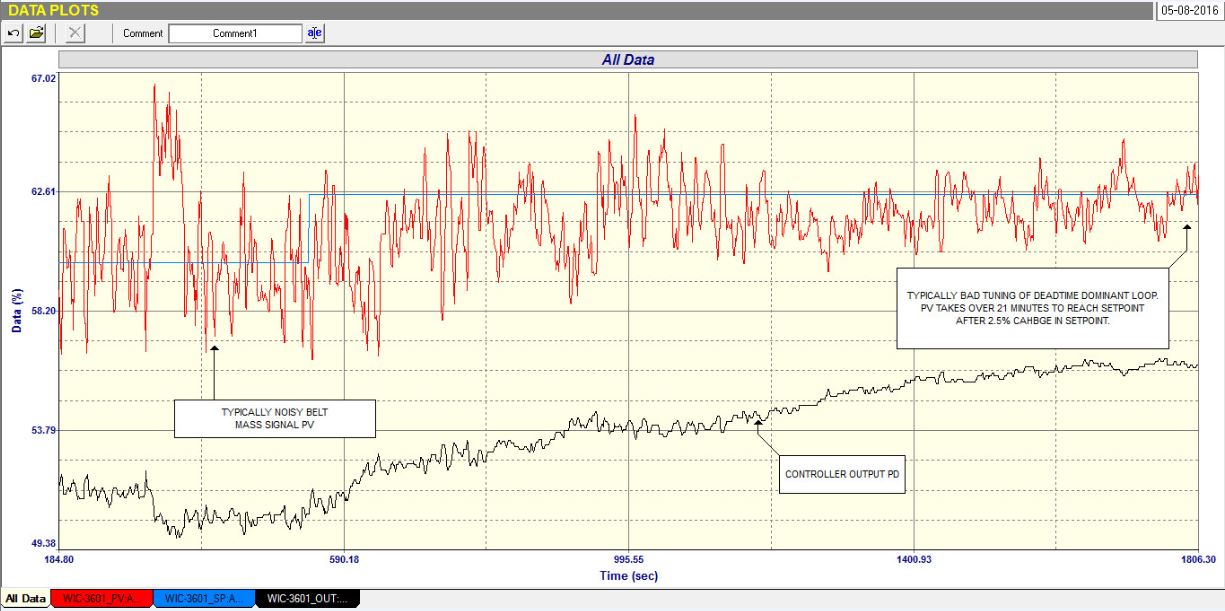
A very good example of this was seen when I was recently performing optimisation at a mine in Portugal. The control was for a weigh feeder. Testing response to input changes on the processes showed that the process had 45 second deadtime. (The lag time constant in the response was effectively zero, making this what is called a true “deadtime only” process, which is practically quite a difficult process to tune if you have not been trained on the methodology, and if you don’t have a proper tuning package that works on such processes.)
Figure 1 is an “as-found” closed loop test, with the original tuning where a 2.5% step change in setpoint was made. It took an unbelievable 22 minutes for the process to get to the new setpoint.
The “as-found” tuning was: P = 0.16, I = 480 seconds/repeat.
Figure 1.
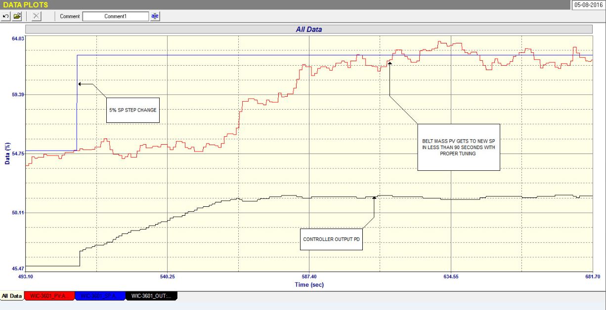
Figure 2 was the final closed loop test with the new tuning. This time a 5% step change in setpoint was made, and it then took just 1.5 minutes for the process to get to the new setpoint. This is about 15 times faster! Also it’s worth while noting what I said earlier: You can normally tune deadtime dominant processes so they can get to new setpoints within two deadtimes.
The new tuning is: P = 0.17, I = 14.6 seconds/repeat.
Figure 2.
This is a very dramatic difference and is a lovely illustration of typically bad tuning of these difficult to control processes.