Home About us Contact us Protuner Loop Analyser & Tuner Educational PDFs Loop Signatures Case Histories
Michael Brown Control Engineering CC
Practical Process Control Training & Loop Optimisation
CONTROL LOOP CASE HISTORY 172
INTERESTING CONTROLS IN A COPPER EXTRACTION PLANT
In my 30 years devoted to optimising controls in industrial process plants in many countries, I thought that I had seen all the possible process dynamics that one would encounter. Imagine my surprise when I came across one I have never encountered before. This was in a temperature control on a plant on a copper smelter plant where I recently presented a course on practical control to process control engineers and also performed some optimisation in a couple of their plants.
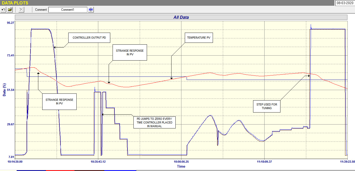
Temperature control optimisation is usually extremely onerous, mainly due to the slowness of the process, and requires a great deal of patience whilst waiting sometimes hours for a process to respond to a step in the controller output (PD) or a change in setpoint (SP). This loop was no different and to make it even more confounding was the fact that the PLC control block had not been set up correctly insomuch that the PD tracking had not been set, so that when the controller was placed in automatic from manual, the controller’s PD should carry on at the same value it had when in manual. Instead it dropped to zero and severely bumped the process. This is incredibly frustrating because it is absolutely necessary to make bumpless changes from automatic to manual and back again when performing optimisation.
Unfortunately no one was present during the work which was done over a weekend who was capable of sorting out the PLC programme, so we had to improvise.
The loop in question was top of the Operators’ problem list. It was in a terrible continuous slow cycle with the PD being either fully open or completely shut and the PV slowly going above or below the setpoint. The Operators had unsuccessfully tried to control the loop in manual, but the problem was that large load changes took place every 20 or 30 minutes when a converter was turned out of stack and emptied. Therefore they had had to leave the loop in automatic, but it was really badly upsetting production. Incidentally this had been like that ever since the plant was built and commissioned 8 years previously.
The process was the temperature control of a cooling heat exchanger. Now heat exchangers normally always have self-regulating dynamics. On starting our tests which had to be mainly performed in manual, we saw that after an hour the PV showed no sign of settling out as normal with a self regulating process, but continued ramping either up or down depending on the magnitude of the PD. I then managed to get hold of a senior process engineer who explained that the process fluid was actually recycled back to the converter’s hood after passing through the exchanger. Therefore after the pass through the hoods, colder water was the coming back to the exchanger cooling it even further. Therefore the process is integrating.
The next thing that I noticed is that every time a step change was made on the PD, the PV responded in a strange way. It firstly slowly curved into the ramp. This normally means that a large lag is present in the process, which is quite normal in temperature processes. However after a while the slope of the ramp curved back into a different slope, which is a very strange response that I had not seen before. This phenomenon can be seen in Figure 1.
Fig 1
After thinking about it I realised that it was a second lag coming back into the PV as the recycled cooling water started coming back into the exchanger. Therefore the dynamics of the process are a slow integrator with a second order lag. This is really unusual dynamics. I have encountered second order lags occasionally on self regulating processes, which is usually a sign of loop interaction, but never on integrating processes.
Fortunately for me the Protuner tunes from a frequency response which it gets by performing a digital Laplace transform over a step change in manual. I strongly believe that no model based tuning system would be able to tune this process, as it would be almost impossible to make a sufficiently accurate model.
The problem here was that we couldn’t get the process into balance due to the PLC problem. Therefore we put the controller into automatic and changed the tuning to P only with a proportional gain of 8. I should mention that the original unstable tuning had P, I and D. Also the derivative filter had been set completely incorrectly. Typical trial and error “desperation” tuning.
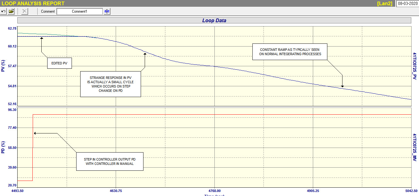
A P only controller is the equivalent of a ball valve on a level control, and automatically finds the balance point. In this case as established later the integral retention time was 1 hour and 10 minutes which is very slow, so it took a long time to try and get the process to near balance, particularly with a few small load changes that were occurring. We got it reasonably close, but unfortunately the operators had to make changes in the process which would have caused a dramatic bump, so we did a step quickly even though we were not exactly at balance. This step can be seen in Figure 2.
Fig 2
We then performed a graphic edit on this PV response to try and get the response to what it may have been if we had actually reached balance. Tuning on this step and then selecting a fairly conservative P+I tune, we first tried it out on the Protuner’s simulator with the process modelled from the frequency plots. It seemed to work well. Also trying the same model with the original tuning exhibited the same instability as originally seen in the loop. Therefore with a great deal of confidence we put this tune into the actual controller and put it into automatic which of course caused the usual huge bump, as the PD went to zero. It then took only about 20 minutes for the loop to get close to setpoint and settle out. It was slightly below setpoint due to the conservative tune, which had an extremely long integral. However within about 30 minutes it reached setpoint and stayed there.
We then ran the control overnight and the next day we saw it had performed extremely well with the load changes. The process manager was really happy to say the least, and said he couldn’t have believed it was possible to have tuned the loop so well.
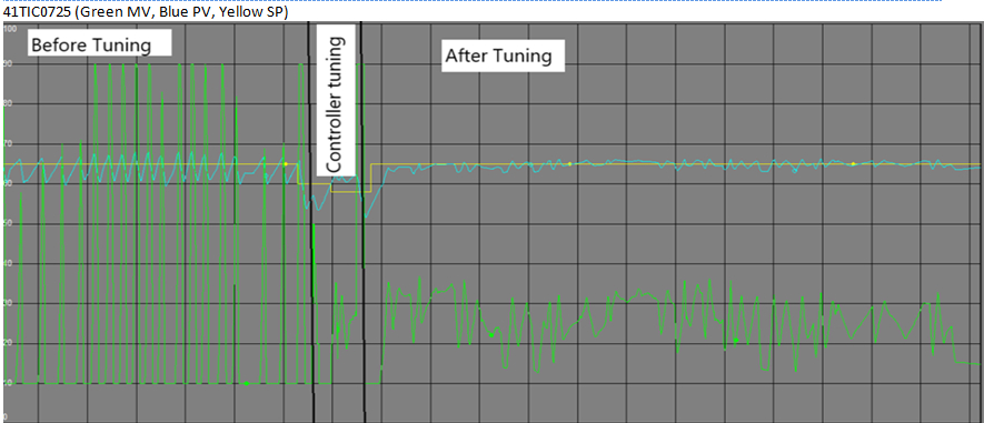
Fig 3
Figure 3 is a screenshot taken from the actual control system’s trends package which shows the performance before and after the optimisation exercise. (The green line is the PD (controller’s output).
All in all, another very successful and pleasurable day at the “coal face”.