Home About us Contact us Training Optimisation Services Protuner Educational PDFs Loop Signatures Case Histories
Michael Brown Control Engineering CC
Practical Process Control Training & Loop Optimisation
LOOP PROBLEM SIGNATURE 1
INTRODUCTION TO "LOOP PROBLEM SIGNATURES" SERIES
Over the years I have had many requests to either write a book, and give more detailed explanations of some of the problems we have encountered in our work on practical loop optimisation. I am by nature and inclination an engineer and not a writer, and have shied away from such a formidable task. Also the publishers of my articles have informed me that they believe that the book would cost more to produce than it would earn, as there is a relatively tiny market for such a work. I also believed that people learn far more, and even more importantly, would gain much better understanding of the subject by actually attending our courses where things are demonstrated by doing exercises on a powerful simulation package, rather than trying to read it up in a book. However some of the past delegates did not have the time and/or opportunity to practice what they had learnt in their plants, and soon forgot much of the course, and many of them have also requested me to put out a book.
To try and meet these requests in a different way, I intend to publish some of the information dealt with in our courses in the next series of articles. Initially the articles will only deal with some of the basics concerning problems and faults commonly encountered in feedback control loops. They will be published under the general heading of "Loop Problem Signatures". It should be noted that many of the things that will appear in this new series of articles may have appeared and been discussed in previous articles dealing with miscellaneous loops in various plants, but the approach here will be to systematically, and sequentially categorise the problems in a more logical approach.
We are also currently planning to open an internet web site hopefully within the next few months, and will also place these articles on the site as they are produced.
To kick off the series and to avoid having to redefine terminology every time an article appears, I will deal with some very basic fundamentals about the feedback loop in this article, and also establish the terminology and names that will be used throughout the series. It is therefore suggested that it would be a good idea to keep this for future reference.
At the outset it should be noted that there are no universal standards and definitions when it comes to industrial instrumentation and control. The industry has been, and will be largely led by the large manufacturers, who generally use their own terminology and definitions. In fact many of them do publish the definitions of all the terms they use in their specifications. Thus it is really important that users are aware of this as one manufacturer may have a different definition of a common term (such as the term 'accuracy' for example), to another manufacturer. It is really a case of "let the buyer beware".
You will therefore appreciate that the terms and names that will be used in these articles may, and most probably will not be the same as those that your instrument manufacturer uses, or which you yourself are familiar with.
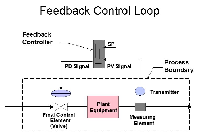
Figure 1
Figure 1 shows a simple feedback control loop. The loop consists of:
* A measuring device (with associated transmitter that converts the signal to a 4 - 20 mA or digital signal which is suitable for transmission back to the control room).
* A final control element, which is often simply called the "valve", even though in actuality it could be any one of a numerous range of devices including dampers, variable speed drives typically powering pumps, fans or belts, louvers, governors, heating appliances, or actual control valves. Although not shown in the figure, the final control element may, and often does, include a current-to-pneumatic (I/P) converter, and a valve positioner.
* A controller.
* Finally the process itself forms an integral and important component of the loop.
From the control point of view however, the process consists of everything external to the controller including the measuring device, transmitter, valve, piping etc. This shown in Figure 1 as the "process boundary".
The signal from the transmitter to the controller will be referred to as "the process variable" (PV), and the signal from the controller to the final control element as "the process demand" (PD). It should be noted that the PV which is one of the input signals to the controller is representing what is happening on the output of the process, whilst the PD which is the output signal from the controller, represents what is happening on the input to the process. This sometimes confuses people, but it will be clearer if you realise that the controller is effectively in parallel with the process.
The controller itself in its simplest form has two inputs. One is called "the setpoint" (SP), which is the value at which you would like to control the process, and the other is the PV which is the actual value of the process. The controller's operation will be discussed in detail in a future series of articles. However for the present, it is important to know that as a general rule, the first thing that a controller does is to subtract the one signal from the other (e.g. "SP-PV"). This difference will be called "the error".
If a process is on setpoint, and is stable, and an error then arises, it will be because either the setpoint, or else the PV has changed. The former is referred to as a "setpoint change", and the latter as a "load change". Load changes are normally caused by external changes which affect the process.
Again in very general terms, in most control loops, the purpose of the controller is to try and keep the error to an absolute minimum. Therefore the best method of being able to determine the effectiveness of the control loop is to calculate the error over a period of time. This will be referred to as "control variance". In reality there are many ways of calculating control variance. For example one could integrate the error over a period of time (say one 8 hour shift). However probably the most commonly used modern method is the use of statistical calculations. The error is sampled at regular intervals (commonly at the controller scan rate). The samples thus obtained are then statistically analysed at longer intervals. The statistical standard deviation gives a good representation of the variance, and is a practice commonly employed in paper manufacture where "2 x Standard Deviation" (commonly referred to as "2 x Sigma"), is used as a measure of the effectiveness of the moisture and basis weight controls on each roll of paper.
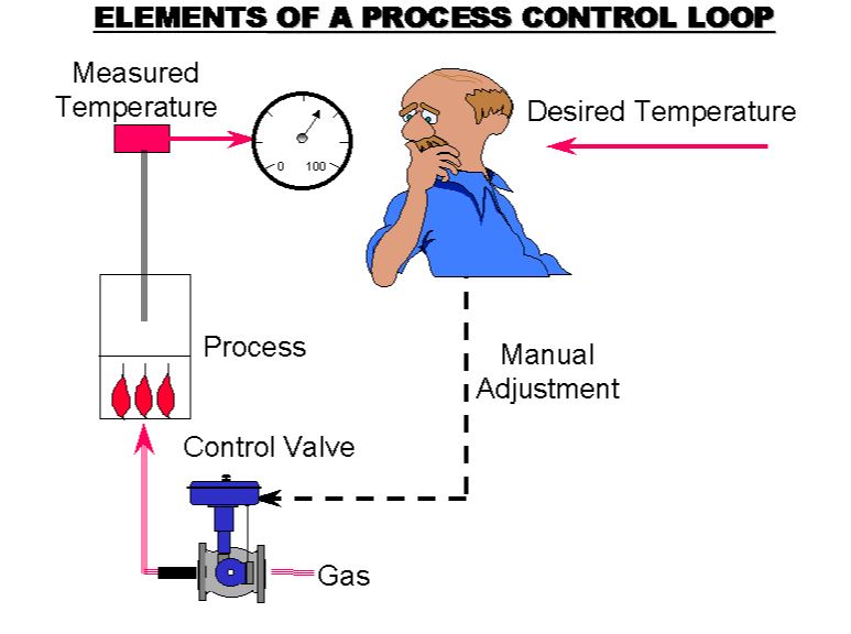
Figure 2.
When operators make changes in manual, they adjust the PD directly, as can be seen in Figure 2.
When working in automatic the controller looks at the error signal, and then solves a mathematical equation. The result of the calculation sets the magnitude of the PD signal. The valve then moves to the position as dictated by the PD which adjusts the amount of whatever is going into the process. The process then reacts accordingly, which will in turn change the value of the PV. This changes the error, and the controller will then recalculate the PD and so on. Thus this sequence is effectively going on round and round the loop on a regular basis (depending on how often the controller does its calculation, which on most modern controllers is once a second).
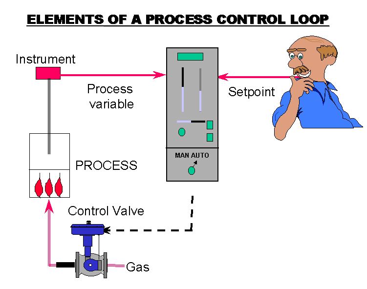
Figure 3
As can be seen in Figure 3, if the control system works efficiently, it would obviously be much easier for the operator to set the desired value on the setpoint on the controller, and let the controller perform all the work of getting the PV to the right value and keeping it there, rather than for him (or her), having to have to do it manually. Unfortunately it is a very sad fact of life that due to the almost complete lack of training (and hence understanding), of the field of truly practical control, the vast majority of control loops are set up so badly that operators generally make most changes in manual rather than in automatic. They usually only leave controllers in automatic when the plant is running under steady state conditions, where of course the controllers are generally doing very little.
Control in automatic is often referred to as "closed loop control", and in manual as "open loop control".
It should be noted that to optimise control loops, one must use at the very minimum, a high speed high resolution, multi-channel recorder. A proper loop analyser like the Protuner which is specifically designed for optimisation work makes the task much easier. It should be noted that the "tools" provided on control equipment like DCS, and SCADA systems are generally completely inadequate for optimisation, particularly for fast processes.
The recorder or analyser, is connected to the process across the controller's input and output (PV and PD signals). Most tests are performed by making changes on the controller either in automatic (closed loop tests), or in manual (open loop tests).
The next article will deal with the two "classes of processes" which is essential to an understanding of practical process control.