Home About us Contact us Protuner Loop Analyser & Tuner Educational PDFs Loop Signatures Case Histories
Michael Brown Control Engineering CC
Practical Process Control Training & Loop Optimisation
LOOP SIGNATURE 24
TUNING - PART 2
SOME "SWAG" METHODS FOR TUNING SIMPLE SELF REGULATING PROCESSES
As mentioned in Part 1 of this series on tuning, it is my opinion that these methods are very crude, and the only reason I am covering them is that they will help give a better understanding of what is involved in tuning, particularly as you progress through this tuning series of articles. They do of course also offer a starting point for tuning, if one is not fortunate enough to have a sophisticated tuning package like a Protuner around.
SWAG Tuning Assumptions
1. The model is a first order lag, deadtime, self-regulating process.
2. Any other process must be “approximated” to this model. (However in reality these simplified methods will not work on processes with complex dynamics).
3. DT<TC
4. Tuning formulae are for a series controller algorithm. (However for P + I only tuning they will also work for the Ideal ISA algorithm. Note that I am only giving formulae for P + I tuning, as any processes where the D term will help in control will have far too complex dynamics to be able to be tuned by SWAG methods. Your really need a sophisticated tuning packet for these).
5. Most tuning is for 1/4 amplitude damped response, which we believe is undesirable. (See appendix at end of article).
Ziegler Nichols Ultimate Sensitivity Tuning
1. Turn off I and D action
2. Start with small P gain (wide PB%).
3. Make a setpoint change and observe the response.
4. Increase the P gain (decrease PB%) in small increments until the loop cycles continuously.
5. Note the P setting (Ku), (ultimate gain), and the period of oscillation (UP) in seconds, (ultimate period).
6. Controller gain: KP = 0.45 x Ku.
7. Controller integral: I = UP/1.2 seconds/repeat.
This method is one of the first tuning methods ever developed. It could effectively be called a simplified frequency response method, insomuch that only one frequency is used, which is the ultimate frequency. Although not perfect, it actually works quite well on simple self-regulating processes. The big disadvantage with it is that you have to put the process into an ultimate cycle, which may not be allowable on many processes.
It gives an insight into the genius of Ziegler and Nichols, when one thinks that all their work that was mostly carried out empirically, using very low accuracy pneumatic measuring instrumentation, and pneumatic circular chart recorders.
There are probably hundreds of different SWAG tuning methods. Why so many? The reason is obvious. If any single method had worked properly, then it would have been universally adapted. Why reinvent the wheel? As none of them did work well universally, people have kept on trying to come up with new ways. Even in the past 10 years new SWAG methods have appeared.
The vast majority of SWAG tuning methods are model based. (See last Loop Signature article for a description of model based tuning methods). Most of them try to determine the process gain (PG), the dead time (DT), and the dominant first order lag (TC), by making a step change in the process. They then “plug” these values into a formula to calculate the tuning parameters. Our experience has been that model based tuning methods are not good. There are various reasons for this, but the main one is that it is extremely difficult to obtain a good model, as small changes in the process dynamics continuously occur in a real operating plant.
Several more sophisticated methods that try and make a far more sophisticated model than a simple first order lag, deadtime model have appeared in recent years. One in particular was developed by the research arm of a large South African chemical company. It was so sophisticated that the model was effectively tested and improved every time a change occurred in the process. The company hailed this as a breakthrough in controller tuning, and there was a great fanfare about it. Eight years after the development it was withdrawn. Basically although the idea was good in principle, it did not work well under actual plant conditions. One of the designers sadly told me that although it worked brilliantly in laboratory conditions, it just could not cope with all the various problems encountered in a real plant.
When modelling from a step test one must be very careful when choosing which step to model from. The following precautions should be taken:
•Tune on only ONE step.
•Tune in manual.
•PV must be constant at start and end of window.
•Avoid steps with possible valve problems (e.g. first step, and steps after valve reversals).
•Tune on step with highest PG, longest DT, fastest TC.
•Add controller scan rate to DT for SWAG tuning.
•Step size of PV should be preferably 10 times bigger than noise amplitude.
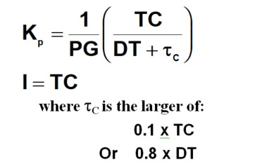
After choosing a step, graphically determine PG, DT, and TC. These dynamics were described in earlier articles in this Loop Signature series. However a diagram showing how to determine them is given in Figure 1 here as a reminder.
Figure 1
Please note that the controller scan rate also adds deadtime into the loop, so for safety sake this should be added to the process deadtime.
Two sets of step response tuning formulae are given:
1. Lambda Model Based Tuning
Controller gain: KP = 1/PG.
Controller integral: I = TC + DT/4 seconds/repeat.
2. IMC Tuning
Of the two sets of formulae, I would suggest that the second (IMC) is the better, but that the integral formulae in the first (Lambda) is better for deadtime dominant processes.
In the next part of this tuning series, we will look at the results of tuning a simple self-regulating process with the three methods given above and also with a couple of other tuning methods.
APPENDIX: Problems with Quarter Wave Response.
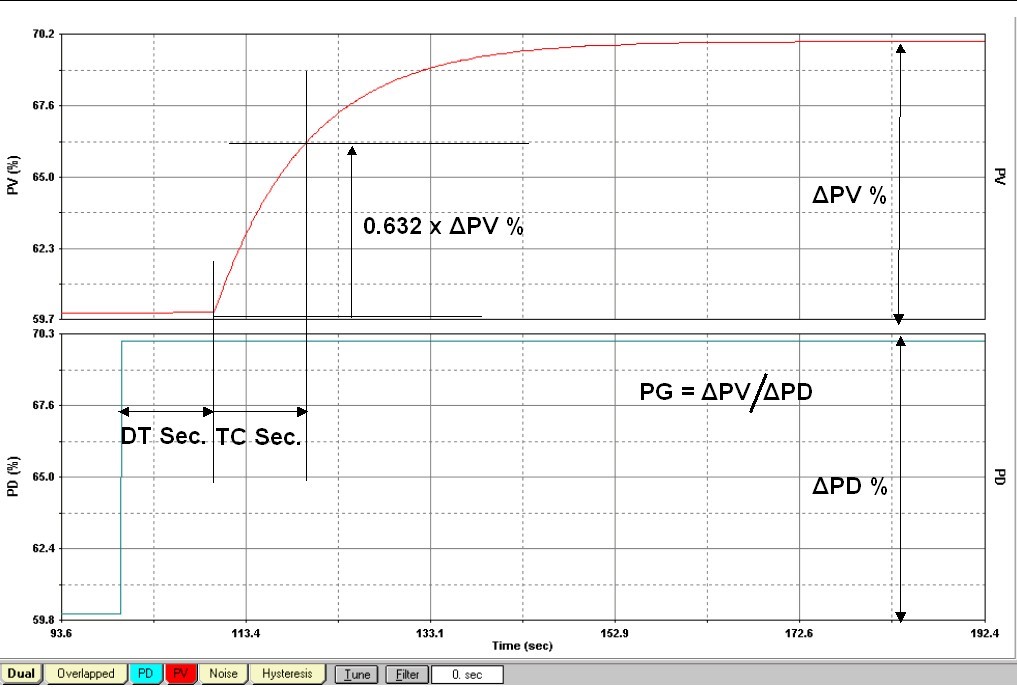
In most control courses one is taught that optimum tuning results in a quarter amplitude damped response, (also called quarter wave damping), to a step change in setpoint. This is because it can be proved that this response gives effectively minimum integrated error. (Sometimes referred to as ISAE tuning). This response is shown in Figure 2.
Figure 2
In reality, optimum tuning for a particular loop depends on all sorts of different criteria. For example the faster you tune a loop, the quicker you wear out the valve. Is this necessary on that particular process, or should the valve be sacrificed for the process? Sometimes you may deliberately wish to have a very slow response for process reasons, etc. A future Loop Signature will cover all the various things that should be taken into account when tuning.
It is our belief that quarter wave damping is not practical or desirable for the following reasons:
1. It is not safe enough, as it does not allow enough gain margin for process dynamic changes, which could result instability.
2. A quarter wave response consists of approximately 4 cycles. This effectively means that the valve has to reverse eight times every time there is a control error change. Is this really desirable? Do you really want to work your valves so hard?
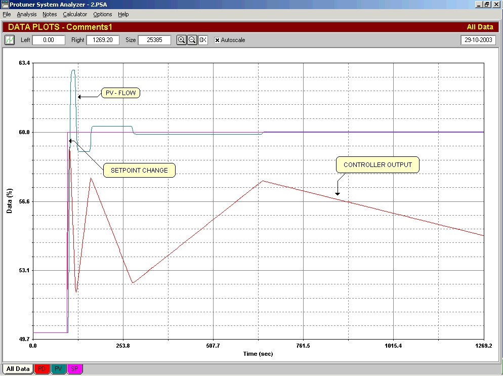
Figure 4
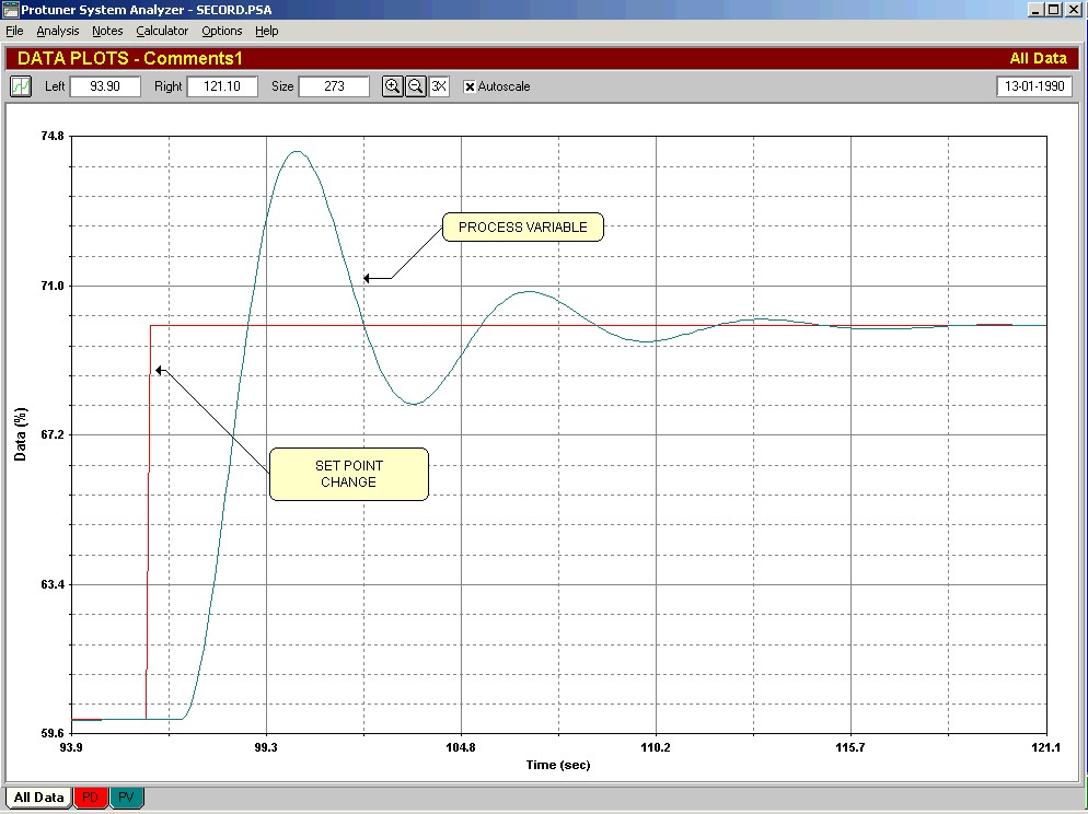
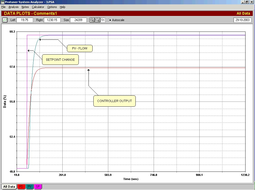
3. As mentioned earlier in this Loop Signature series, most valves suffer from a certain amount of hysteresis. As shown there, it means that on each reversal of the valve the controller output has to ramp through the hysteresis band under the command of the controller’s integrator. This slows down the control, and increases variance. On a slow process like temperature it can literally take hours before the process finally settles out. This means that in reality on many, if not most loops, quarter amplitude damped tuning probably results in much worse control variance than even critical damping, where no valve reversals at all are made on a control error change. Figure 3 shows the first part of the response on a step change in setpoint on a flow loop with quarter wave damping. There is 5% hysteresis on the valve. Note the loop is still trying to get to setpoint after about 20 minutes. Figure 4 shows the same loop with critical damping. Its settles out in a few seconds!
4. As can be seen in Figure 2, it would be very hard actually judge a quarter amplitude damped response in real control equipment, where the screens normally do not have great resolution on the tuning trends.
5. In real life in nearly every plant I have been in, at least 85% of the loops are tuned probably at least a magnitude slower than quarter amplitude damping.
This would indicate to me that in fact quarter amplitude damping is unrealistic and impractical. If a fast response is required on a loop I normally tune it to give a single overshoot. This increases the gain margin by over 100% from quarter amplitude damped responses, which makes it much safer. In general I find the new response is generally anything from about 4 to 2000 times faster than the “as found” tuning.