Home About us Contact us Protuner Loop Analyser & Tuner Educational PDFs Loop Signatures Case Histories
Michael Brown Control Engineering CC
Practical Process Control Training & Loop Optimisation
LOOP PROBLEM SIGNATURE 3
PROCESS DYNAMICS - PROCESS GAIN
An instrumentation technician once told me that to him a process consists only of a trace on a screen. This is rather a sad attitude. If one wishes to control a process then it is important to have a reasonable basic knowledge and understanding of the process itself, and certainly one should also be aware of what external influences can act on it. To this end, if you are not intimately familiar with the process yourself, it is essential that you work with a process expert who can guide and help you in gaining this understanding. Apart from this, if you wish to successfully optimise the control of a process, it is also essential that you establish the dynamics of the process.
Process dynamics are described by an equation known as the process transfer function, which can be loosely described as various factors which cause the output of the process to respond in a particular way to any change on the input of the process. The importance of understanding the dynamics of any process is fundamental to successful control optimisation, and cannot be overstressed. In our control optimisation courses, process dynamics occupies a large part of the more advanced part of the course. Unfortunately all this information is beyond the scope of these articles, and only a few of the more basic factors will be covered, viz. process gain, deadtime, and single first order lags. It is of interest to note that these three factors were, and largely still are, the only factors that are taken into account in many of the more simplistic tuning techniques, (for example, Ziegler & Nicholls tuning), which is one of the reasons why these tuning methods often fail, as there are also many other dynamic factors that may occur in real process responses.
In this article we will deal with process gain, firstly for self regulating processes, and secondly for integrating processes.
Fig 1.
Figure 1 shows a simple pressure control self regulating loop. The controller is in manual, and a step change is made on the output of the controller (process demand - PD). The pressure (process variable - PV), rises up exponentially and settles out at a new value. The process gain is defined as the size of the step in PV, measured after it has reached steady state, divided by the size of the step that was made in the PD. The measurements are made in percent of span, and as these units cancel, process gain of a self regulating process is unitless. It is also sometimes referred to as loop forward gain, or steady state gain. It can be thought of as an amplification factor in the process.
In practice the process gain is very important. It is made up by two factors, the first being the valve sizing, and the second the spanning of the transmitter. Ideally one would like to use the full span of both devices, particularly that of the valve, which being a mechanical devices is very limited in rangeability, and may suffer from problems like hysteresis and backlash. Therefore if the valve was moved from 0 - 100% open operating position, and the measurement responded likewise from 0 - 100%, then the process gain would be unity, which is ideal.
As a general rule of thumb, if the process gain is greater than unity the valve is oversized, and if it is less than unity, it is usually due to the transmitter span being too wide.
One disadvantages of a valve being oversized is that the proportional gain in the controller has to be correspondingly reduced to achieve a desired response. This leads to problems on many controllers that have limited low end gains. Typically many commercial controllers are limited to a minimum gain of 0.1 (or 1000% proportional band). On fast processes like flows, which are tuned with low gain and fast integral, it may not be possible to set a low enough gain in the controller if the valve is oversized.
Another and probably even more important disadvantage of oversized valves is that the process gain actually amplifies the valve imperfections, and results in a degradation of control performance. Therefore if a valve suffers from say a 1% hysteresis (which is pretty normal), the offset as seen on the PV will be that 1% offset multiplied by the process gain. For example if we had a process gain of 4, then the offset on the PV would be 4%. This means that the control error also becomes bigger in a directly proportional relationship to the valve oversizing. Also if a cycle occurs in closed loop due to a valve problem, like a hysteresis cycle on an integrating loop, then the amplitude of the cycle as seen on the PV, will also be multiplied by the process gain.
On the other side, if a transmitter is spanned too wide which results in a process a gain of less than unity, problems can occur firstly with the quality of the measurement. For example if the process gain was 0.5, it would mean that only the first 50% of the transmitter span was being used. If this was on say an orifice flow, it would severely limit the useful flow range and measurement accuracy.
Secondly a low process gain also necessitates having to increase the controller proportional gain to achieve a particular control response. This makes the output of the controller more "jumpy", and will also further amplify signal noise which results in increased valve wear and possibly increased control variance.
As a general rule of thumb, good engineering practice dictates that the process gain for a self regulating process should lie between 0.5 and 2.0.
Fig 2.
Figure 2 shows an open loop test performed in a South African petrochemical refinery, on a flow control valve that was hugely oversized. The process gain in this case was close to 13! The valve itself had negligible hysteresis and as a result, in this particular case, good control could in fact be achieved. However to realise this, the proportional gain that had to be inserted in the controller was 0.000125 (or proportional band of 8,000%)!
Process gain for an integrating loop is rather different. As explained in the last article in this series, the PV can only be constant in an integrating process when the PD is at the balance point. Once the PD moves off balance the, PV starts ramping.
One way of defining the process gain for an integrating level loop would be the as the slope of the PV ramp resulting when the PD is at 100%, and there is zero flow out of (or into, as the case may be), the other side of the tank.
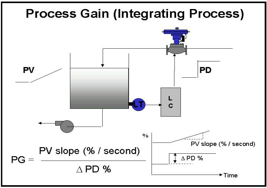
Fig 3.
Figure 3 shows how the process gain is measured in practice for such a process. The unit of process gain for an integrating process is "inverse seconds". (It is a slope).
The reciprocal of the process gain for a level process, is known as the tank retention time. This is the time that it would take for the tank to empty from full to zero if there was no flow into the other side of the tank. As most tanks would take a considerable time to empty, it becomes apparent that the process gain of most integrating processes, will be tiny numbers, generally much, much, smaller than unity. For example if the retention time of a tank was 1,000 seconds, its process gain would be 0.001.
Therefore in light of this, another fact becomes immediately apparent, and this that if fast control is required for an integrating processes, in most cases, one is going to need relatively high proportional gains in the controller to counter the small process gains.