Home About us Contact us Training Optimisation Services Protuner Educational PDFs Loop Signatures Case Histories
Michael Brown Control Engineering CC
Practical Process Control Training & Loop Optimisation
Loop Problem Signatures Part 2 - 19
DYNAMICS OF MORE COMPLEX PROCESSES
SLOW "PURE" INTEGRATORS
A couple of years ago in my course on difficult processes, I used to tell the delegates that I would teach them about every dynamic they were ever likely to encounter in real life process control. However a year or so ago, I was invited to spend a couple of days helping two of them optimising controls in their plant which manufactured chipboards. It was there that I came across a new variety of dynamic that I had not encountered before. This was on a loop that controlled temperature on platens in a board press.
A platten is effectively a large metal slab with internal ducts through which hot oil is passed. It is placed between boards that are being pressed under high pressure. Good temperature control is very important, or the boards will warp and will be spoilt. When we started on this loop I looked at the existing tuning parameters that had been set in the controller, and nearly fell off my chair, because the proportional gain had been set to a value of 150.
I have never seen such a high gain in a controller before. It is close to ON/OFF control, which as everyone knows is unstable with the process moving in a continuous cycle. I said as much to the engineers at the plant, but they replied that it seemed to work quite well. On testing the system, I did indeed find it was stable and operating very well. How could this be the case? An investigation was needed.
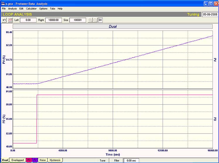
The first step was to perform an open loop test on the system to establish the dynamics, which is shown in Figure 1. The response of the process to a step change on the controller output indicated that it was a fairly simple integrating process with a transfer function of:
Where PG is the process gain, and DT is the deadtime. (S is the Laplace operator).
Fig. 1
This was covered pretty well in Loop Signature Part 2-16, which, was published a few months ago. This type of process is normally highly susceptible to instability, and initially it was extremely puzzling as to how one could have such a high gain in the controller, without putting the loop into a cycle.
It should also be also be noted that it could be clearly seen in Figure 1 that there is no lag in the process, as the ramp section of the response started immediately without “curving up” into the ramp, which is the characteristic of a lag on an integrating process (see Loop Signature P2-17).
A full analysis of the response gave the following dynamic constants:
PG (Process Gain) = 0.00006 per second.
DT (Deadtime) = 68 seconds.
In the dynamics of the simple first order lag, deadtime, self-regulating processes, discussed in early articles in this Part 2 Loop Signature series, it may be remembered that the ratio between deadtime and time constant was called “the controllability factor” for self-regulating processes, and was very important. In particular the bigger it got, the more difficult the control became, and visa-versa, the smaller it became, the easier it was to control, and in fact in Loop Signature P2-11, it was shown that if the deadtime was less than a tenth of the time constant, then the process could be considered “a pure lag”, which is almost impossible to go unstable whatever the tuning, and in practice one could get away with relatively huge gains in the controller without problem, resulting in much faster responses.
Now this was with self –regulating processes, but it does appear that an equivalent relationship may apply to simple integrating processes with no lag and only deadtime, but the relationship here lies between the amount of deadtime, and the process gain.
This sounds very strange, but it should be remembered from Loop Signature LS3 (available on my CD “Basic Trouble Shooting and Loop Tuning – available to readers outside Southern Africa) that the process gain of an integrating process is essentially the slope of the steepest ramp that can be obtained on the process - for example, in the case of a level process where the vessel was filling or emptying at the fastest possible rate, and slope is related to time – typically slope is measured in “%/second”. Now in the aforementioned article it was shown that the reciprocal of the process gain is equal to the retention time of the tank. So if the retention time is measured in seconds, the process gain is given in the reciprocal of time, i.e. “per second”.
Another thing that can also be considered logical is that the smaller the process gain (i.e. the longer the retention time), the higher the proportional gain that can be placed in the controller without the loop becoming unstable). As an extreme example consider the control of the level in a swimming pool. When the level drops because of evaporation, one would never consider restoring the level by using a modulating controller. You would merely fully open the tap of the water supply, and then close it when the level was restored. This is ON/OFF control and is in reality quite stable in this case. ON/OFF control has infinite proportional gain (or zero proportional band). Alternatively as we know, fast level processes with small retention times are more difficult to control, and can easily go unstable. These types of processes are normally tuned with relatively much smaller proportional gains. However, if there is very little deadtime in the process, then again the control is not so difficult.
This leads to an understanding that the relationship between deadtime and process gain is very important when it comes to control of an integrating process.
In general we can now say that the ratio of deadtime to retention time could be regarded as the “controllability factor” for integrating processes. The smaller it is, the easier it is to control the process, and visa versa, the larger, the more difficult it is to control the process.
As in the case of deadtime versus time constant for self regulating processes, then similarly for integrating processes, there must be a point where the ratio between deadtime and process gain can be regarded as allowing one to insert virtually any tuning in the controller without worrying about instability. Numerous tests carried out have shown that when DT< 0.03/PG, or DT<0.03xRetention Time, then one can treat this as a pure integrator, where the deadtime will have little effect on stability.
Where will one encounter pure integrators in practice? To date I personally have encountered this type of dynamics on extremely slow temperature processes that do not have a first order lag, like the platen temperature control system described earlier. Level controls on tanks with very long retention times can also have similar dynamics. However one could never ever put really extremely high gains into controllers on levels, as level measurement is always noisy.
How does one go about tuning a pure integrator? Firstly be aware that with the peculiar properties that integrating processes display when tuned with P and I as discussed in Loop Signature P2-16, the I term can have a significant effect on instability. Even with a pure integrator, too fast an integral term in the controller can result in cyclic responses. Therefore the following procedure is recommended:
Start with P only tuning, and increase the P value until you get the fastest response you desire. This will involve taking the following two factors into account:
- 1. Unless the deadtime is truly negligible, then, even on a P only controller, with sufficiently high enough gains, it will eventually be possible to get the response to start cycling, and even reach instability. Therefore as a eneral rule try and avoid more than a single overshoot, or even tune for critical damping, which is the highest gain one can use before the process will start overshooting on a setpoint change.
- 2. It should be noted that even with a very tiny noise on the PV signal (which is normal for temperature signals due to the large inherent filtering effect provided by the thermowell), a high gain in the controller can cause the valve to start jumping around, as the noise will be amplified by the gain and will appear on the output of the controller. This may shorten the life of the valve. In a case like this, a filter (which should be as small as possible) can be placed on the PV to dampen the noise.
With a high proportional gain in the controller, any offset should be very small. (Remember that the maximum possible offset with a P only controller will be about half of the proportional band of the controller). However if it were not acceptable then an integral term would have to be used in the controller. This can be calculated from the little formula given in Loop Signature P2-16.
It should be remembered, that as mentioned in that Loop Signature, P only control for an integrating process is in fact superior to P+I control for several reasons. However in real life, people do not like offset, so P+I is generally always used.
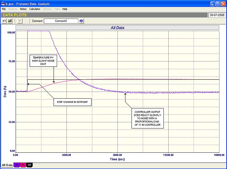
The loop for which the open loop test was performed as shown in Figure 1 was tuned with normal tuning criteria. The Protuner gave a Proportional Gain of 11, and an Integral setting of 7,378 seconds/repeat.
A closed loop step test with these parameters is shown in Figure 2. It can be seen that the response to the step change in setpoint was quite good with a slight overshoot that took along time to recover. (Remember from Loop Signature P2-16, that using the I term on an integrating process will always result in overshoot on setpoint step changes). In addition there was a tiny noise of 0.1% amplitude on the temperature PV signal. This does slightly affect the PD output as it is amplified through the Proportional gain factor.
Fig. 2
The deadtime in this process is 68 seconds, and the process gain is 0.00006, which is really small. (The retention time is 4.6 hours). 0.03/PG gives a value of 500. Therefore as the deadtime is so much less, the process can definitely be treated as a pure integrator.
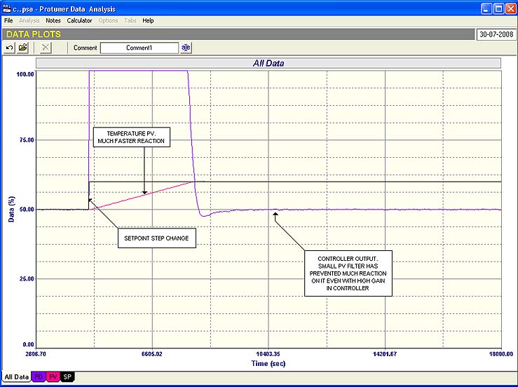
Trial by error tuning with P only control resulted in a P gain of 80 giving a nice fast response without overshoot. Although a maximum offset of only ±0.5% maximum is possible with such a high gain (tiny proportional band), it was decided to add an integral term to eliminate any offset. The use of the above-mentioned formula resulted in an I term of 833 seconds/repeat.
A proportional gain of 80 amplifying the noise would result in severe valve oscillation, even with such minute noise amplitude. Therefore a filter of 30 seconds was placed before the PV to reduce the noise to virtually zero. A 30 second filter is relatively tiny on a slow process like this, and will not have any detrimental effects.
The final closed loop test with the new tuning is shown in Figure 3. It can be seen what a vast improvement in response the new tuning has given.
Fig. 3
This is a good example that shows how important it is to identify specific cases of dynamics when doing tuning, so that optimum tuning can be applied.